Dollar Cost Averaging vs. Lump Sum Investments

# Import everything we need
import datetime
import random

%matplotlib inline
import matplotlib.pyplot as plt
import numpy as np
from yahoo_finance import Share

# Create a quote object to make later code a bit more readable.
# I prefer not to index into a dict everytime I need the closing
# price of a stock.
class Quote(object):
    def __init__(self, quote_dict):
        self.symbol = quote_dict['Symbol']
        self.date = datetime.datetime.strptime(quote_dict['Date'], '%Y-%m-%d').date()
        self.high = float(quote_dict['High'])
        self.low = float(quote_dict['Low'])
        self.open = float(quote_dict['Open'])
        self.close = float(quote_dict['Close'])
        self.adj_close = float(quote_dict['Adj_Close'])
        self.volume = int(quote_dict['Volume'])

    def __repr__(self):
        return '<Quote {} {}>'.format(self.symbol, self.date)

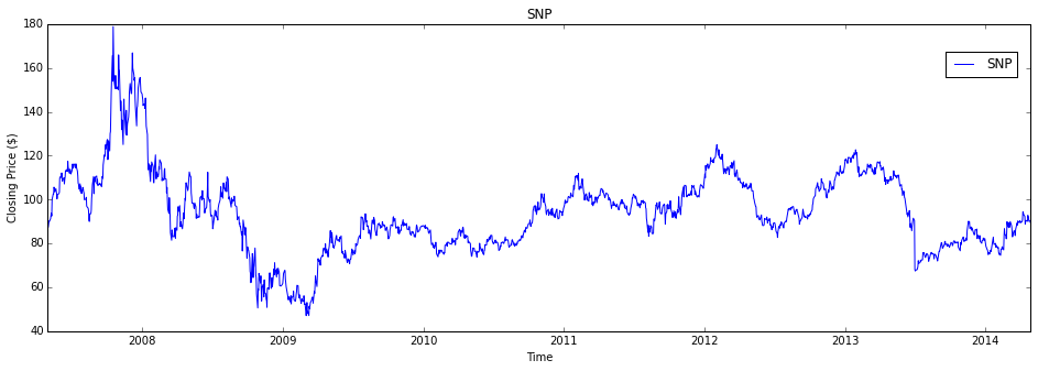
# Let's define the stock and the range of
# stock history that we are interested in
stock_ticker_symbol = 'SNP'
start, end = '2007-04-30', '2014-04-29'

# Get the data and sort it.
stock = Share(stock_ticker_symbol)
stock_history = stock.get_historical(start, end)
stock_history = [Quote(q) for q in stock_history]
stock_history.sort(key=lambda q: q.date)

# Number of days of stock history
days = len(stock_history)
days

1763

plt.subplots(figsize=(16,5))
plt.plot([q.date for q in stock_history], [q.close for q in stock_history],
         label=stock_ticker_symbol)
plt.title(stock_ticker_symbol)
plt.xlabel('Time')
plt.ylabel('Closing Price ($)')
plt.legend(bbox_to_anchor=(0, 0.85, 1, 0.102), loc=1, ncol=1, borderaxespad=1)
plt.show()

Lump Sum Purchase

Let's take a look at the case where we invest a dollar for each day of stock history that we have. However we invest all of that money up front on the first day of our stock history.

# Price on day 0
stock_history[0].close

87.21

# If I bought (number of days from start to end) dollars worth of
# shares on day 0, I'd have this many shares:
dollars_invested = days
shares = dollars_invested / stock_history[0].close
shares

20.215571608760463

for day in stock_history:
    # let's take note of how much our holdings
    # are on each day so we can make a graph
    day.lmp_holdings_value = shares * day.close

# Price on last day
stock_history[-1].close

89.36

# If I sold all my shares on the last day,
# I'd have this much cash:
holdings_value = shares * stock_history[-1].close
holdings_value

1806.463478958835

# Thus my ROI would be:
(holdings_value - dollars_invested) / dollars_invested

0.02465313610824442

Dollar Cost Averaging

Now let's take a look at a similar case (where we invest a dollar for each day of stock history that we have) but instead of investing all of the money upfront, we invest one dollar on each day of our stock history.

total_shares = 0
for day in stock_history:
    # Buy one dollar's worth of shares each day
    shares_per_dollar = 1 / day.close
    total_shares += shares_per_dollar
    # let's take note of how much our holdings
    # are on this day so we can make a graph
    day.dca_holdings_value = total_shares * day.close

# On the last day, I'd have this many shares
total_shares

19.52774974818405

# On the last day, I'd have this much cash
holdings_value = stock_history[-1].dca_holdings_value
holdings_value

1744.9997174977266

# Thus my ROI would be:
(holdings_value - dollars_invested) / dollars_invested

-0.010210029780075678

plt.subplots(figsize=(16,5))
plt.plot([q.date for q in stock_history], [q.lmp_holdings_value for q in stock_history], label="Lump Sum")
plt.plot([q.date for q in stock_history], [q.dca_holdings_value for q in stock_history], label="Dollar Cost Averaging")
plt.title('Value of holdings vs. Time')
plt.xlabel('Time')
plt.ylabel('Closing Price ($)')
plt.legend(bbox_to_anchor=(0, 0.88, 1, 0.102), loc=1, ncol=3, borderaxespad=1)
plt.show()

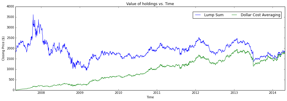
Conclusions Thus Far

I'm not super impressed by DCA. From what I've seen above, the DCA strategy seems slow and not that performant.

My question now is, did I pick a bad start date for my interval of history? If I picked a different start date and ran the same equations over that interval of history and prices, would I see different results? The question that follows is, how many different start dates would I have to try before I saw the DCA strategy out perform the lump sum strategy? How about all of them? How about I try starting my stock history on each day of the real stock history. We'll keep the ends of each stock history interval pinned to the last day of the real stock history. That would give me "days" intervals to check.

For example:

Interval 1: start day = day 0 of stock history
Interval 2: start day = day 1 of stock history

# Let's create a function to calculate the ROI values for
# both strategy's for a given start date.

def get_roi(start_day=None):
    """
    Determine the performance of the lump sum method of investing
    vs. the dollar cost averaging method. Start investing from
    start_day which is an index into the list of days of stock history.

    If start_day is not given, choose a random day in between the
    end and the beginning of stock_history.
    """
    start_day = start_day if start_day is not None else random.randint(0, days - 1)
    interval_history = stock_history[start_day:]
    num_of_days = len(interval_history)

    # Lump Sum Method
    price_on_day_0 = interval_history[0].close
    dollars_invested = num_of_days
    shares_purchased = dollars_invested / interval_history[0].close
    dollars_on_last_day = shares_purchased * interval_history[-1].close
    lump_sum_roi = (dollars_on_last_day - dollars_invested) / dollars_invested

    # Dollar Cost Averaging
    shares_purchased = 0
    dollars_to_invest_per_day = dollars_invested / num_of_days
    for day in interval_history:
        shares_purchased += dollars_to_invest_per_day / day.close
    dollars_on_last_day = shares_purchased * interval_history[-1].close
    dca_roi = (dollars_on_last_day - dollars_invested) / dollars_invested

    return lump_sum_roi, dca_roi

# Lets compare each strategy's ROI for each possible
# investment start date in our real stock history.
dca_better_than_lump_count, intervals = 0, days
for day in range(intervals):
    lump, dca = get_roi(day)
    if dca > lump:
        dca_better_than_lump_count += 1

# Percentage of time the DCA method out performed the lump sum method
(dca_better_than_lump_count / intervals) * 100

52.07033465683494

Wow! 52% of the time, DCA's ROI is greater than lump sum's strategy. I'd still like to see how that's possible. Maybe a graph will help.

# Let's get those same ROI numbers from before, convert
# them to percentages, and then plot them.
lumps, dcas = [], []
for day_index in range(len(stock_history)):
    lump, dca = get_roi(day_index)
    lumps.append(lump * 100)
    dcas.append(dca * 100)

plt.subplots(figsize=(16,5))
plt.plot([q.date for q in stock_history], [lumps[i] for i in range(days)], label="Lump Sum")
plt.plot([q.date for q in stock_history], [dcas[i] for i in range(days)], label="Dollar Cost Averaging")
plt.title('% ROI vs. Investment Start Date')
plt.xlabel('Investment Start Date')
plt.ylabel('ROI (%)')
plt.legend(bbox_to_anchor=(0, 0.88, 1, 0.102), loc=1, ncol=1, borderaxespad=1)
plt.show()

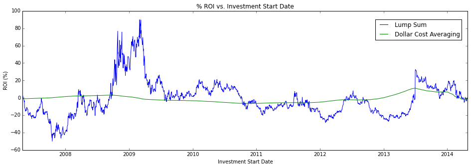
Wow! This graph says a lot. For a given investment start date, we can see the ROI for each investment strategy. Dollar cost averaging really gives us a great deal of security while investing in any market conditions. Our money doesn't really seem to grow much via the DCA strategy but it also doesn't shrink much at all. Compared with the lump sum strategy, the DCA strategy introduces almost zero risk due to "investing at the wrong time".

So what is DCA good for? From what I can tell, dollar cost averaging is a techinque to safely invest in the stock market. We take on much less risk of loosing value because the market has gone down by investing via the DCA strategy. We won't really gain much value, if any, from bull markets but we won't loose much value from bear markets either. So why do value investors encourage the use of DCA? I assume they plan to make their money on the dividends; more reaserch to be done.